6.00.2x学习笔记Week4
Understanding Experimental Data
现实中对实验结果的测量有很多无法避免的因素影响结果的准确性。Computation可以帮助我们把这些影响降低到最低,以便得到更加准确的实验结果。
- 做一个假设,如果我做x,y会发生。
- 设计一个实验,并测量实验结果
上述两者有时候可以转换
- 有了结果之后,要拿结果进行运算
- 是否可以证明假设的结论
- 求出假设中的那个未知系数的值
- 如果假设能够被实验证明,那就可以做预测了
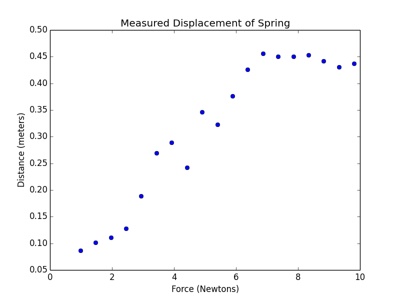
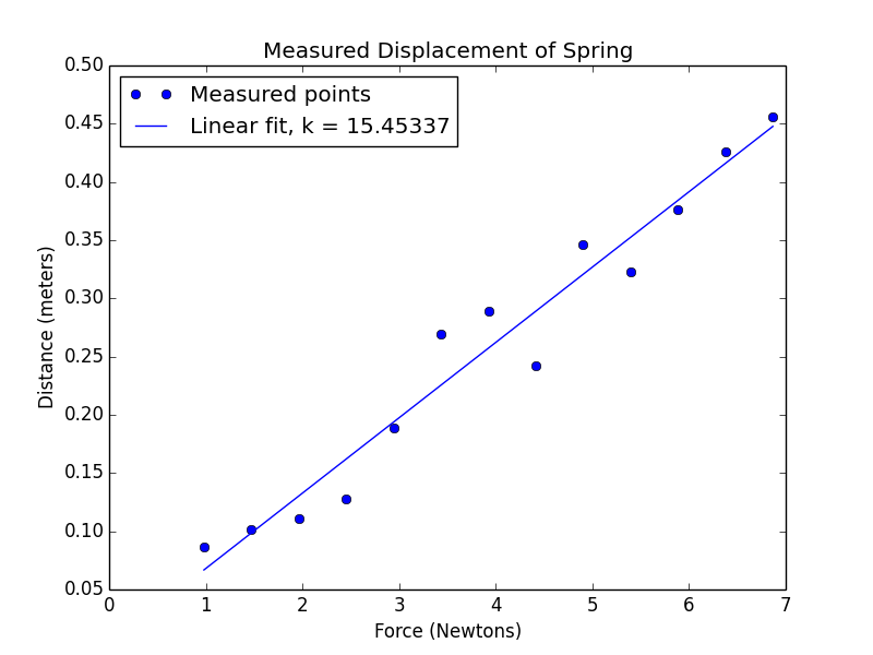
在弹簧拉伸实验中,每次悬挂不同重量的石块,计算出来的弹簧系数都不同。我们把数据plot出来看一下能否找出什么规律。
import pylab, random

def getData(fileName):
    dataFile = open(fileName, 'r')
    distances = []
    masses = []
    discardHeader = dataFile.readline() #去掉第一行
    for line in dataFile:
        d, m = line.split()
        distances.append(float(d))
        masses.append(float(m))
    dataFile.close()
    return (masses, distances)

def plotData(fileName):
    xVals, yVals = getData(fileName)
    xVals = pylab.array(xVals)
    yVals = pylab.array(yVals)
    xVals = xVals*9.81 # convert mass to force (F = mg)
    pylab.plot(xVals, yVals, 'bo', label = 'Measured displacements')
    pylab.title('Measured Displacement of Spring')
    pylab.xlabel('Force (Newtons)')
    pylab.ylabel('Distance (meters)')

plotData('springData.txt')
pylab.show()
实验中的error是很多随机的小错误的集合。
def testErrors(ntrials=10000,npts=100):
    results = [0] * ntrials
    for i in xrange(ntrials):
        s = 0   # sum of random points
        for j in xrange(npts):
            s += random.triangular(-1,1)
        results[i] =s
    # plot results in a histogram
    pylab.hist(results,bins=50)
    pylab.title('Sum of 100 random points -- Triangular PDF (10,000 trials)')
    pylab.xlabel('Sum')
    pylab.ylabel('Number of trials')

testErrors()
pylab.show()
Probability Density Function
在[-1,1]中随机取100个数,他们的和在[-100,100]之间。做10000次这样的实验,把他们的和做成histgram。
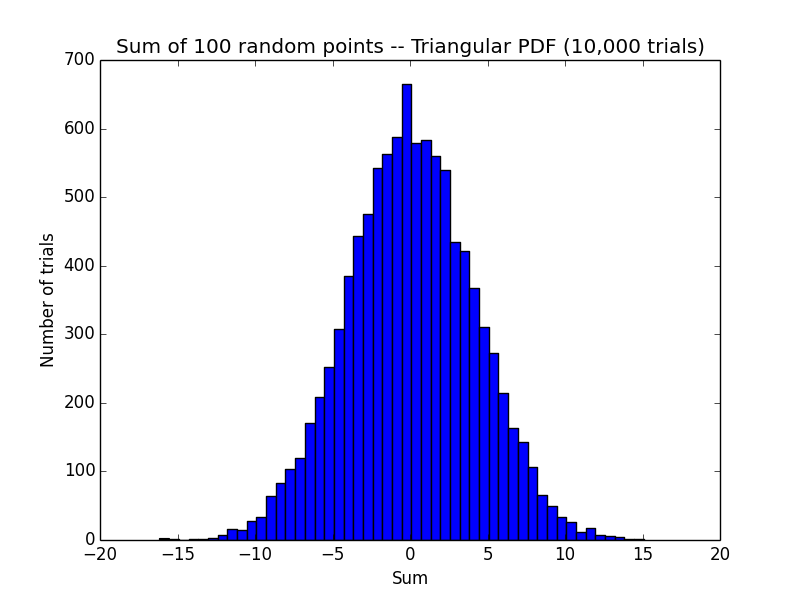
random.triangular(low, high, mode) Return a random floating point number N such that low <= N <= high and with the specified mode between those bounds. The low and high bounds default to zero and one. The mode argument defaults to the midpoint between the bounds, giving a symmetric distribution.
这里说明,多做实验可以让影响结果的错误相互抵消。
把Observation与Prediction之间的距离看成是error。
选择prediction的参数,就是把(obs-pred)2最小化。这被称作SSE(Sum of square of Errors)。又被称作Least Squares。
用pylab.polyfit(xVals, yVals, 1)求得SSE的最小参数a并绘制成一条直线。
def fitData(fileName):
    xVals, yVals = getData(fileName)
    xVals = pylab.array(xVals)
    yVals = pylab.array(yVals)
    xVals = xVals*9.81  # convert mass to force (F = mg)
    pylab.plot(xVals, yVals, 'bo', label = 'Measured points')
    pylab.title('Measured Displacement of Spring')
    pylab.xlabel('Force (Newtons)')
    pylab.ylabel('Distance (meters)')
    a,b = pylab.polyfit(xVals, yVals, 1)  # fit y = ax + b
    # use line equation to graph predicted values
    estYVals = a*xVals + b
    k = 1/a
    pylab.plot(xVals, estYVals, label = 'Linear fit, k = '
               + str(round(k, 5)))
    pylab.legend(loc = 'best')

fitData('springData.txt')
pylab.show()

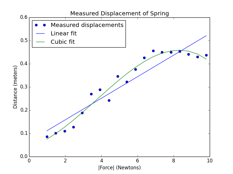
但这看上去不像是最合适的fit。如果用立方关系来绘制曲线pylab.polyfit(xVals, yVals, 3),得到这样的结果。
def fitData1(fileName):
    xVals, yVals = getData(fileName)
    xVals = pylab.array(xVals)
    yVals = pylab.array(yVals)
    xVals = xVals*9.81  # convert mass to force (F = mg)
    pylab.plot(xVals, yVals, 'bo', label = 'Measured displacements')
    pylab.title('Measured Displacement of Spring')
    pylab.xlabel('|Force| (Newtons)')
    pylab.ylabel('Distance (meters)')
    a,b = pylab.polyfit(xVals, yVals, 1)
    estYVals = a*xVals + b
    pylab.plot(xVals, estYVals, label = 'Linear fit')
    a,b,c,d = pylab.polyfit(xVals, yVals, 3)
    estYVals = a*(xVals**3) + b*xVals**2 + c*xVals + d
    pylab.plot(xVals, estYVals, label = 'Cubic fit')
    pylab.legend(loc = 'best')

fitData1('springData.txt')
pylab.show()
但是如果继续用Terman’s law来做预测。得到了这样不可能的结果。
def fitData2(fileName):
    xVals, yVals = getData(fileName)
    extX = pylab.array(xVals + [1.05, 1.1, 1.15, 1.2, 1.25])
    xVals = pylab.array(xVals)
    yVals = pylab.array(yVals)
    xVals = xVals*9.81  # convert mass to force (F = mg)
    extX = extX*9.81    # convert mass to force (F = mg)
    pylab.plot(xVals, yVals, 'bo', label = 'Measured displacements')
    pylab.title('Measured Displacement of Spring')
    pylab.xlabel('|Force| (Newtons)')
    pylab.ylabel('Distance (meters)')
    a,b = pylab.polyfit(xVals, yVals, 1)
    estYVals = a*extX + b
    pylab.plot(extX, estYVals, label = 'Linear fit')
    a,b,c,d = pylab.polyfit(xVals, yVals, 3)
    estYVals = a*(extX**3) + b*extX**2 + c*extX + d
    pylab.plot(extX, estYVals, label = 'Cubic fit')
    pylab.legend(loc = 'best')

fitData2('springData.txt')
pylab.show()
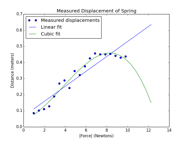
得到了这样不可能的结果。这时如果我们再去看Hooke’s law的观测结果。发现最后几个点几乎在一条直线上,也就是弹簧不再伸长了。也就是说Hooke’s达到了弹簧伸缩的极限。如果我们把最后6个点去掉再来制图。
def fitData3(fileName):
    xVals, yVals = getData(fileName)
    xVals = pylab.array(xVals[:-6])
    yVals = pylab.array(yVals[:-6])
    xVals = xVals*9.81  # convert mass to force (F = mg)
    pylab.plot(xVals, yVals, 'bo', label = 'Measured points')
    pylab.title('Measured Displacement of Spring')
    pylab.xlabel('Force (Newtons)')
    pylab.ylabel('Distance (meters)')
    a,b = pylab.polyfit(xVals, yVals, 1)  # fix y = ax + b
    # use line equation to graph predicted values
    estYVals = a*xVals + b
    k = 1/a
    pylab.plot(xVals, estYVals, label = 'Linear fit, k = '
               + str(round(k, 5)))
    pylab.legend(loc = 'best')

fitData3('springData.txt')
pylab.show()
得到了这样的曲线。这就与观测非常的吻合了。但这时又带来一个问题,我们能随意去掉不符合预测的观测结果吗?这里有一个假设,就是弹簧有弹性极限,过了一个特定的点,就不再伸长了。
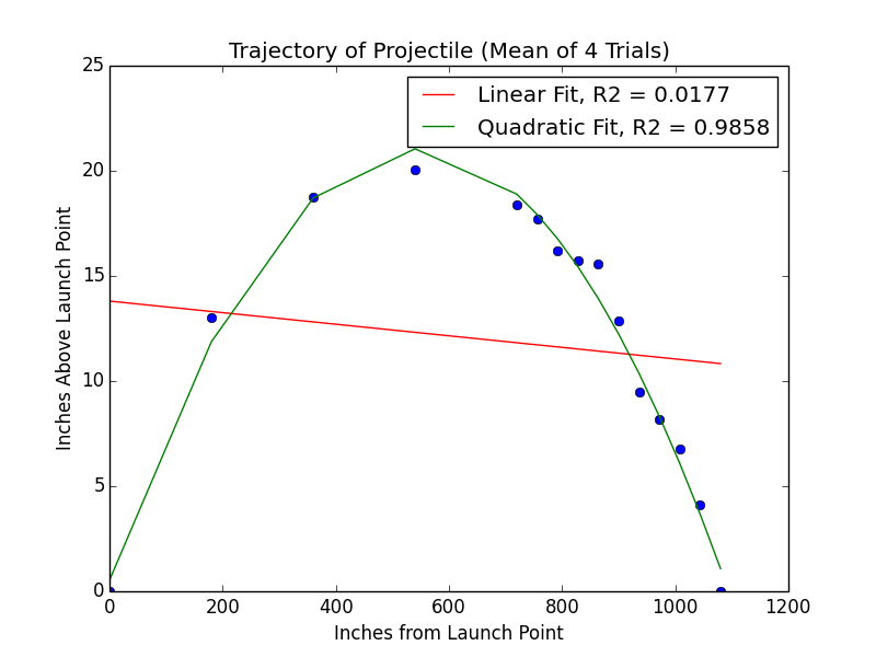
我们再研究弓箭射出的曲线。弓箭射出后,不同时间点离地面的高度。看能否用数学公式来表示弓箭的飞行线路。我们还会看一下如何确定我们的预测曲线与实际观测是否吻合的方法,因为之前我们只是通过肉眼观察。也就是用数学方法来确定预测与观测之间的吻合程度。
def getTrajectoryData(fileName):
    dataFile = open(fileName, 'r')
    distances = []
    heights1, heights2, heights3, heights4 = [],[],[],[]
    discardHeader = dataFile.readline()
    for line in dataFile:
        d, h1, h2, h3, h4 = line.split()
        distances.append(float(d))
        heights1.append(float(h1))
        heights2.append(float(h2))
        heights3.append(float(h3))
        heights4.append(float(h4))
    dataFile.close()
    return (distances, [heights1, heights2, heights3, heights4])

def tryFits(fName):
    distances, heights = getTrajectoryData(fName)
    distances = pylab.array(distances)*36
    totHeights = pylab.array([0]*len(distances))
    for h in heights:
        totHeights = totHeights + pylab.array(h)
    pylab.title('Trajectory of Projectile (Mean of 4 Trials)')
    pylab.xlabel('Inches from Launch Point')
    pylab.ylabel('Inches Above Launch Point')
    meanHeights = totHeights/float(len(heights))
    pylab.plot(distances, meanHeights, 'bo')
    a,b = pylab.polyfit(distances, meanHeights, 1)
    altitudes = a*distances + b
    pylab.plot(distances, altitudes, 'r',
               label = 'Linear Fit')
    a,b,c = pylab.polyfit(distances, meanHeights, 2)
    altitudes = a*(distances**2) + b*distances + c
    pylab.plot(distances, altitudes, 'g',
               label = 'Quadratic Fit')
    pylab.legend()

tryFits('launcherData.txt')
pylab.show()

显然,平方关系与观测结果更吻合。但是如何用数学语言描述呢?这要提到variability of errors。
compare the variability of errors to the variability of the original data.
这时我们用到统计学上的一个概念,叫做决定系数(coefficient of determination),有的教材上翻译为判定系数,也称为拟合优度。当R2接近1,说明model和数据更接近,如果R2接近0,则说明偏差很大。
用代码表示:
def rSquare(measured, estimated):
    """measured: one dimensional array of measured values
       estimate: one dimensional array of predicted values"""
    SEE = ((estimated - measured)**2).sum()
    mMean = measured.sum()/float(len(measured))
    MV = ((mMean - measured)**2).sum()
    return 1 - SEE/MV
把Coefficient of determination加入到刚刚的制图中。
def tryFits1(fName):
    distances, heights = getTrajectoryData(fName)
    distances = pylab.array(distances)*36
    totHeights = pylab.array([0]*len(distances))
    for h in heights:
        totHeights = totHeights + pylab.array(h)
    pylab.title('Trajectory of Projectile (Mean of 4 Trials)')
    pylab.xlabel('Inches from Launch Point')
    pylab.ylabel('Inches Above Launch Point')
    meanHeights = totHeights/float(len(heights))
    pylab.plot(distances, meanHeights, 'bo')
    a,b = pylab.polyfit(distances, meanHeights, 1)
    altitudes = a*distances + b
    pylab.plot(distances, altitudes, 'r',
               label = 'Linear Fit' + ', R2 = '
               + str(round(rSquare(meanHeights, altitudes), 4)))
    a,b,c = pylab.polyfit(distances, meanHeights, 2)
    altitudes = a*(distances**2) + b*distances + c
    pylab.plot(distances, altitudes, 'g',
               label = 'Quadratic Fit' + ', R2 = '
               + str(round(rSquare(meanHeights, altitudes), 4)))
    pylab.legend()

tryFits1('launcherData.txt')
pylab.show()
这里要注意的是:
A model that explains every single point of data without error might be overfitting the data, which would not provide accurate description of the process behind the data.
建模的意义在于很多实验没法做,例如核反应堆冷却失效。既然我们了解了弓箭的抛物线模型的数学公式,如果有人问我需要多厚的盾来保护自己,我们看一下怎么做。
要做这个计算,首先要把弓箭的速度算出来。
Read more: